On this page, we’ll visualize the geodesic flow from previous sections with two perspective shifts. This section involves knowledge of point-set topology, group presentations, and group actions.

(Currently, the animations in this section use some set of “generators” which don’t actually generate a Fuchsian group. We are working on constructing these animations using a representation of the surface group of a genus \(2\) surface in \(\text{PSL}(2, \mathbb{R})\).)

Fundamental Domains as Quotients of Fuchsian Groups

In the toral automorphism section, we saw that the fundamental domain for a torus in the Euclidean plane was a unit square. Consider the group \(G\) generated by the translations \((x, y) \mapsto (x + 1, y)\) and \((x, y) \mapsto (x, y + 1)\). For any \(g \in G\) and \(p \in \mathbb{R}^2\), consider the action of \(G\) on \(\mathbb{R}^2\) defined by \[g \cdot (x, y) = g(x, y).\] For any \((x, y) \in \mathbb{R}^2\), \[G \cdot (x, y) = \{(x + m, y + n) : m, n \in \mathbb{Z}\}.\] Most importantly, note that for any coset \(S\) in \(\mathbb{R}^2/G\), there exists a unique respresentative of \(S\) in the unit square with opposite sides identified. In fact, there is a homeomorphism between \(\mathbb{R}^2/G\) and the unit square with opposite sides identified. It is in this sense that the notions of

• the torus as a \(2\)-dimensional surface embedded in \(3\)-dimensions,
• the unit square with opposite sides identified, and
• \(\mathbb{R}^2/G\)

are all different perspectives on the same object. (Some may recognize that \(G \cong \mathbb{Z}^2\) is the fundamental group of the torus.)

We can make a similar perspective shift for hyperbolic surfaces. An important object will be the set of distance-preserving maps of the hyperbolic plane.

Isometries: A map \(f : \mathbb{H}^2 \to \mathbb{H}^2\) is called an isometry (of \(\mathbb{H}^2\)) if for all \(p, q \in \mathbb{H}^2\), \[d(p, q) = d(f(q), f(q)),\] where \(d\) is the standard hyperbolic metric on \(\mathbb{H}^2\). In other words, an isometry is a distance-preserving map.¹ The set of isometries of \(\mathbb{H}^2\) is denoted \(\text{Isom}(\mathbb{H}^2)\), which is a group under function composition.

Important: The reason why \(\text{Isom}(\mathbb{H}^2)\) is important is the following theorem: every hyperbolic surface is the quotient of the hyperbolic plane \(\mathbb{H}^2\) by a particular kind of subgroup of \(\text{Isom}(\mathbb{H}^2)\). Such subgroups are known as Fuchsian groups.²

Consider the Poincaré half-plane, representing the points as complex numbers. It turns out that every isometry of \(\mathbb{H}^2\) is given by a linear fractional transformation³, which, in this context, is an invertible map \(\mathbb{H}^2 \to \mathbb{H}^2\) given by \[z \mapsto \frac{az + b}{cz + d},\] where \(a, b, c, d \in \mathbb{R}\). We can identify such a transformation as a matrix \(\begin{pmatrix} a & b \\ c & d \end{pmatrix}\). This is natural because composition of linear fractional transformations corresponds to multiplication of matrices under this identification.

But two matrices that differ by the multiplication of a nonzero scalar correspond to the same linear fractional transformation. So, if we want to represent the linear fractional transformations as some set of matrices, what we’re really looking at is:⁴ \[\text{GL}(2, \mathbb{R})/\{\lambda \in \mathbb{R} - \{0\}\} \cong \text{SL}(2, \mathbb{R})/\{I, -I\} \cong \text{PSL}(2, \mathbb{R}),\] where \(\text{SL}(2, \mathbb{R})\) is the set of \(2 \times 2\) real matrices with determinant \(1\), and \(\text{PSL}(2, \mathbb{R})\) is defined by the second homomorphism.

The Point: Anyways, the point is: \[\text{Isom}(\mathbb{H}^2) \cong \text{PSL}(2, \mathbb{R}),\] where elements in the latter, which look like \[\left\{\begin{pmatrix} a & b \\ c & d \end{pmatrix}, -\begin{pmatrix} a & b \\ c & d \end{pmatrix}\right\}\] with \(a, b, c, d \in \mathbb{R}\) and \(ad - bc = 1\), are acting on \(\mathbb{H}^2\) by the corresponding linear fractional transformations.

Consider a genus \(g\) surface, \(S_g\). There is an important group associated with any topological space, known as the fundamental group. The fundamental group of \(S_g\) (denoted \(\pi(S_g)\)) is given by \[\pi(S_g) = \langle a_1, b_1, a_2, b_2, \dots, a_g, b_g \mid [a_1, b_1] [a_2, b_2] \cdots [a_g, b_g] = e \rangle,\] where \([a_i, b_i] = a_i b_i a_i^{-1} b_i^{-1}\).

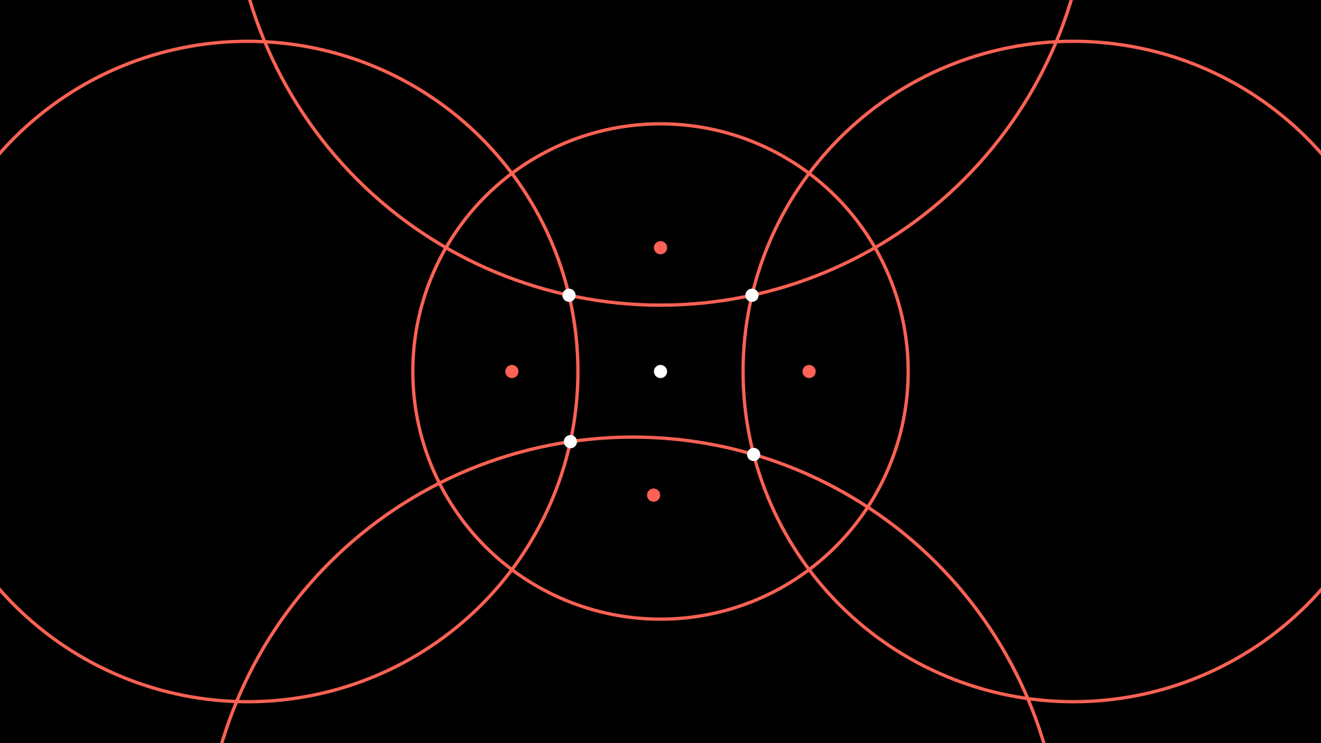
Here’s the main idea: just like how \(G \leq \text{Isom}(\mathbb{R}^2)\) and \(G \cong \mathbb{Z}^2 \cong \pi(S_2)\), we’ll have some subgroup \(\Gamma \leq \text{Isom}(\mathbb{H}^2)\) such that \(\Gamma \cong \pi(S_g)\). And just like how the unit square with opposite sides identified allowed us to visualize \(\mathbb{R}^2/G\), we will be looking for a region in \(\mathbb{H}^2\) that allows us to visualize \[\mathbb{H}^2/\Gamma.\] Luckily, there’s a mechanical process of doing so, called a Dirichlet domain. Working in the Poincare disk, consider a starting point \(z\), say, in the center of the circle. For each generator \(s\) of \(\Gamma\) (in the case of \(\Gamma = S_g\), \(s \in \{a_1, b_1, \dots, a_g, b_g\}\)), act on \(z\) by \(s\) and \(s^{-1}\); that is, draw the points \(s \cdot z\) and \(s^{-1} \cdot z\):

In Euclidean geometry, if we have two points \(A\) and \(B\), there is a line \(\ell\) such that \(\ell\) passes through the midpoint of \(\overline{AB}\) and \(\ell \perp \overline{AB}\).

Similarly, if we have two points \(p, q \in \mathbb{H}^2\), define \(\ell_{pq}\) to be the geodesic in \(\mathbb{H}^2\) that is perpendicular to the geodesic between \(p\) and \(q\) and passes through the midpoint of \(p\) and \(q\), where distances are measured using the hyperbolic metric of the Poincaré disk. For each of the new points \(p\), draw \(\ell_{zp}\) (which will be a Euclidean circle):

And the region containing \(z\) turns out to be a fundamental domain for \(\mathbb{H}^2/\Gamma\)!

We want to animate the geodesic flow in this fundamental domain, as in previous sections. But the geodesic flow corresponding to a point with an associated unit vector in the Poincaré disk might move outside of the Dirichlet domain after some time. So, we need an algorithm that takes any point \(p\) in the disk and finds its corresponding element in the Dirichlet domain (that is, the element in the Dirichlet domain that is in the same coset in \(\mathbb{H}^2/\Gamma\) as \(P\)).

Representation Finding Algorithm: Start with some point \(p\) in the Poincaré disk.

1. Apply each of the generators and their inverses to \(p\) to generate a set of new points \(S\).
2. If no point in \(S\) is closer to \(z\) than \(p\), then \(p\) is in the Dirichlet domain, and stop the algorithm.
3. Otherwise, consider the set \(S'\) of points in \(S\) that are closer to \(z\) than \(p\). Replace \(p\) with the point in \(S'\) that is closest to \(z\).
4. Repeat starting from step \(1\).

The following image depicts this algorithm, where we scattered many random blue dots in the disk, and plotted their corresponding point in the Dirichlet domain as a green dot:

The Unit Tangent Bundle

We’ve successfully shifted one of our perspective to Fuchsian groups, and used Dirichlet domains to recover corresponding fundamental domains. But even in the image above, we would still have to pick a point and a unit vector in order to actually represent a geodesic flow. Instead, defining \(S^1 = \{z \in \mathbb{C} : |z| = 1\}\) to be the unit circle, define the unit tangent bundle \[T^1 \mathbb{H}^2 = \mathbb{H} \times S^1,\] which basically just bundles points and unit vectors together. There’s also a topology on \(T^1 \mathbb{H}^2\), which formally defines the following intuition we would want the space to have: if \(p, q \in \mathbb{H}^2\) are close together and \(v, w \in S^1\) are close together, then \((p, v)\) and \((q, w)\) are close together in \(T^1 \mathbb{H}^2\).

Previously, we looked at how linear fractional transformations act on \(\mathbb{H}^2\). The derivative of a linear fractional transformation \[f : z \mapsto \frac{az + b}{cz + d}\] with \(ad - bc = 1\) is given by \[f' : z \mapsto -\frac{a(cz + d) - c(az + b)}{(cz + d)^2} = -\frac{1}{(cz + d)^2},\] which is how linear fractional transformations act on unit vectors (treating them as complex numbers with magnitude \(1\)).

It turns out that for each element \((p, v) \in T^1 \mathbb{H}^2\), there exists a unique linear fractional transformation \(l\) such that \[l \cdot (i, i) = (p, v).\] This means that we can identify \(T^1 \mathbb{H}^2\) with linear fractional transformations, by saying that every point in \(T^1 \mathbb{H}^2\) corresponds to the linear fractional transformation that sends \((i, i)\) to that point.

But it is also a fact that for any matrix \(M \in \text{SL}(2, \mathbb{R})\), we can decompose it into matrices of the form⁵ \[M = \begin{pmatrix} \cos{\theta} & -\sin{\theta} \\ \sin{\theta} & \cos{\theta} \end{pmatrix} \begin{pmatrix} r & 0 \\ 0 & \frac{1}{r} \end{pmatrix} \begin{pmatrix} 1 & x \\ 0 & 1 \end{pmatrix},\] where \(\theta \in [0, 2\pi)\), \(r \in (0, \infty)\), and \(x \in \mathbb{R}\). This gives us three parameters: one that corresponds to a circle, and two that correspond to the Poincaré half-plane under the map \[(r, x) \mapsto x + \frac{1}{r^2} i,\] which preserves the geometry of the situation. We can transform this Poincaré half plane into the Poincaré disk using a Cayley transformation. In total, we have a circle parameter and a disk parameter, which corresponds to a solid torus.

Under this identification of \(\text{SL}(2, \mathbb{R})\) with a solid torus, elements of \(\text{PSL}(2, \mathbb{R}) \cong T^1 \mathbb{H}^2\) correspond to pairs of points. The following animation depicts the geodesic flow of several sample pairs of points in \(\text{PSL}(2, \mathbb{R})\), where two points of the same color are paired together.

(Note: While it appears that some of the spherical dots are not entirely contained in the torus towards the end of the animation, this is because the center of the dot is extremely close to the boundary of the torus.)

Finally, using the results of this paper⁶, we observed that the fundamental domain for the geodesic flow on the unit tangent bundle of a surface, under this identification with the torus, can be found by rotating the fundamental domain we found using Dirichlet domains along the \(\theta\) parameter. That is, a slice of the torus-like object in the following animation corresponds to a Dirichlet domain, as shown.

This animates the geodesic flow corresponding to a Fuchsian group, and the algorithm works given any Fuchsian group in terms of elements of \(\text{PSL}(2, \mathbb{R})\) as an input.

However, part of the overarching goal of this project is to visualize geodesic flow in the context of the more general notion of hyperbolic groups. In full generality, it’s difficult to animate aspects of these geodesic flows in only three dimensions, and figuring out how to observe information about geodesic flows from visualizations of this general case is something we hope to explore in the future.

References