Lie Algebra Cohomology

This tool computes Lie algebra cohomology of certain Lie algebra representations by Kostant’s version of the Borel-Weil-Bott theorem.

It is a partial recreation of Josef Silhan’s (non-functional as of October 2025) website created for this purpose at https://web.math.muni.cz/~silhan/lie/.

Background

Let \(\mathfrak{g}\) be a simple Lie algebra of highest weight \(\mu\) with a fixed parabolic subalgebra \(\mathfrak{p}\le \mathfrak{g}\). This induces a grading \(\mathfrak{g}=\mathfrak{g}_{-k}\oplus \cdots \mathfrak{g}_k\) of \(\mathfrak{g}\) for which \(\mathfrak{p}=\mathfrak{g}_0\oplus \cdots \oplus \mathfrak{g}_k.\) Let \(\mathfrak{g}_-=\mathfrak{g}_{-k}\oplus \cdots \oplus \mathfrak{g}_{-1}\). Let \(\mathfrak{g} \curvearrowright V\) be an irreducible representation of lowest weight \(-\lambda\). Then there is an action by \(\mathfrak{g}_0\) on the Lie algebra cohomologies \(H^k(\mathfrak{g}_-,V).\) Let \(W^{\mathfrak{p}}\subset W\) be the Hasse diagram associated to \(\mathfrak{p},\) let \(W^{\mathfrak{p}}_{(k)}\subset W^{\mathfrak{p}}\) be the subset of elements of length \(k\), and let \(\cdot\) be the affine action by the Weyl group on weights given by \(w\cdot \sigma=w(\sigma+\rho)-\rho.\) Then according to Borel-Weil-Bott theorem, \(H^k(\mathfrak{g}_-,V)\cong \bigoplus_{w\in W^{\mathfrak{p}}_{(k)}}V^{w \cdot \lambda}\) where \(V^{\sigma}\) is the \(\mathfrak{g}_0\) irreducible representation of lowest weight \(-\sigma.\)

Given \(\mathfrak{p}\le \mathfrak{g},\) our program computes the Hasse diagram \(W^{\mathfrak{p}}\) and the orbit of \(\lambda\) under the affine action by \(W^{\mathfrak{p}}.\) This orbit gives all the minus lowest weights of the \(\mathfrak{g}_0\) irreducible subrepresentations of \(H^k(\mathfrak{g}_-,V).\)

In the case where \(V=\mathfrak{g}\) under the adjoint representation, we can also compute an integer gradation associated to each \(\mathfrak{g}_0\) irreducible component of \(H^k(\mathfrak{g}_-,\mathfrak{g})\).

Using the Tool

Dynkin Diagram Orientations

We use the following Dynkin diagrams:

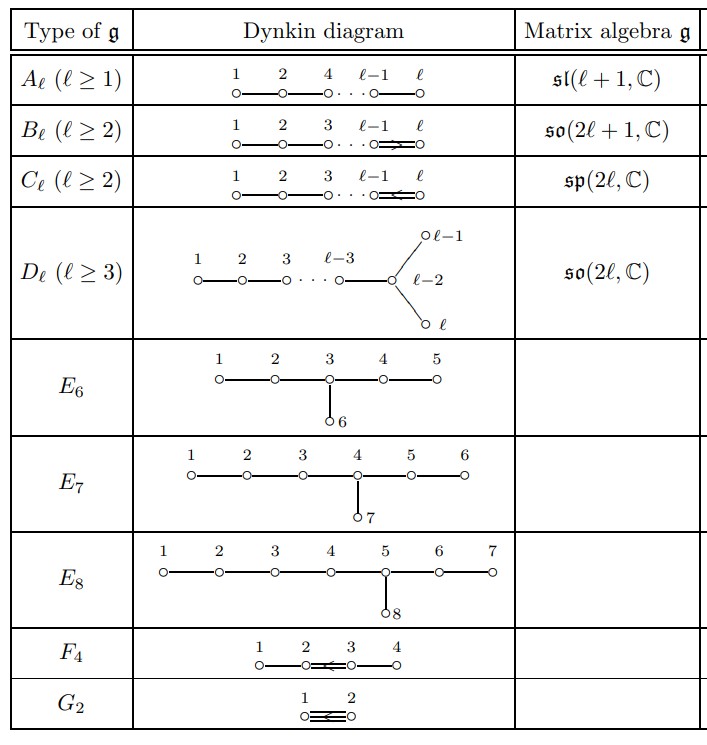
Image credit: A. Čap and J. Slovák.